STA 243 Computational Statistics
Discussion 7: Python: Gradient Descent Methods for Quadratic Minimization Problem
TA: Tesi Xiao
Let us start with a qudratic minimization problem in $\mathbb{R}^2$.
\[\min_{x\in \mathbb{R}^2} ~ \frac{1}{2} (x-x^\star)^\top A (x-x^\star)\]Assume $x^\star=0$ for simplicity. The gradient and Hessian of $f(x)$ are given by
\[\nabla f(x) = Ax, \nabla^2 f(x) = A.\]In addition, assume $A$ is positive definite. Then, one can easily show that $f(x)$ is $\lambda_{\min}(A)$-stongly convex and $\lambda_{\max}(A)$-smooth.
The condition number of $A$: $\kappa(A) = \lambda_{\max}(A)/\lambda_{\min}(A)$
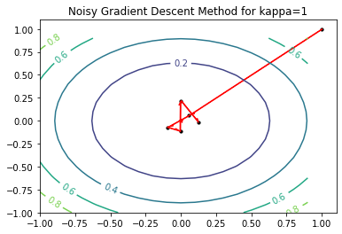
The GD, Heavy Ball, Nestrov’s accelerated GD, SGD methods are implemented below. Note that the update of SGD for solving the problem above uses the noisy gradient information, i.e., $g(x_t) = \nabla f(x_t) + \epsilon, \epsilon\sim N(0, \sigma^2)$.
Gradient Descent Method:
\[x_{t+1} = x_t - \eta \nabla f(x_t)\]Convergence: $\eta = \frac{2}{\lambda_{\max}(A) + \lambda_{\min}(A)},\quad \Vert x_{t+1} - x^\star \Vert_2^2 \leq \frac{\kappa-1}{\kappa+1} \Vert x_t - x^\star \Vert_2^2$
Heavy Ball Method:
\[x_{t+1} = x_t - \eta \nabla f(x_t) + \gamma (x_t - x_{t-1})\]Convergence: $\eta = \frac{4}{(\sqrt{\lambda_{\max}(A)} + \sqrt{\lambda_{\min}(A)})^2}, \gamma = (\frac{\sqrt{\kappa}-1}{\sqrt{\kappa}+1})^2, \quad \Vert x_{t+1} - x^\star \Vert_2^2 \leq \frac{\sqrt{\kappa}-1}{\sqrt{\kappa}+1} \Vert x_t - x^\star \Vert_2^2$
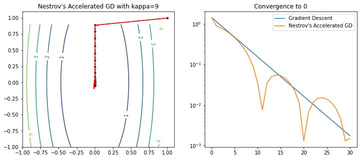
Nestrov’s Accelerated GD Method:
\[x_{t+1} = y_t - \eta \nabla f(y_t), \quad y_{t+1} = x_{t+1} + \frac{t}{t + 3} (x_{t+1} - x_t)\]Convergence: In the convex setting (not strongly convex), $\eta = \frac{1}{L}, \quad f(x_t) - f^\star = c/t^2$.
import numpy as np
import matplotlib.pyplot as plt
class quadratic_function(object):

    def __init__(self, d=2, A=None, xstar=None):
        self.d = d
        if A is None:
            A = np.random.rand(d,d)
            A = A.T @ A
        if xstar is None:
            xstar = np.zeros(d)
        self.A = A
        self.xstar = xstar

    def fun_value(self, x):
        return (x-self.xstar).T @ self.A @ (x-self.xstar)/2

    def grad_value(self, x):
        return self.A @ (x - self.xstar)
class ALG(object):

    def __init__(self, fun, x0):
        self.fun = fun
        self.x = x0
        self.trajectory = [x0.copy()]
        self.t = 0

    def update(self):
        pass

class GD(ALG):

    def __init__(self, fun, x0):
        ALG.__init__(self, fun, x0)

    def update(self, eta):
        self.x -= eta*self.fun.grad_value(self.x)
        self.trajectory.append(self.x.copy())
        self.t += 1


class HeavyBall(ALG):

    def __init__(self, fun, x0):
        ALG.__init__(self, fun, x0)

    def update(self, eta, gamma):
        if self.t == 0:
            self.x -= eta*self.fun.grad_value(self.x)
        else:
            self.x -= eta*self.fun.grad_value(self.x) - gamma*(self.x - self.trajectory[-2])
        self.trajectory.append(self.x.copy())
        self.t += 1

class NestrovAcc(ALG):

    def __init__(self, fun, x0):
        ALG.__init__(self, fun, x0)
        self.y = x0

    def update(self, eta):
        self.x = self.y - eta*self.fun.grad_value(self.y)
        self.y = self.x + self.t/(self.t + 3) * (self.x - self.trajectory[-1])
        self.trajectory.append(self.x.copy())
        self.t += 1

class SGD(ALG):

    def __init__(self, fun, x0):
        ALG.__init__(self, fun, x0)

    def update(self, eta, sigma=1):
        self.x -= eta* (self.fun.grad_value(self.x) + np.random.normal(scale=sigma, size=self.fun.d))
        self.trajectory.append(self.x.copy())
        self.t += 1
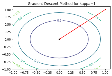
We start with applying GD to the problem where $A=I$. Thus, $f(x_1, x_2) = (x_1^2+x_2^2)/2, \kappa = 1$. Setting $x_0 = [1,1]^\top$ and $\eta = 1$, GD can find $x^\star$ with 1 step.
f = quadratic_function(d=2, A=np.array(([1,0],[0,1])))
alg = GD(f, x0=np.array([1.,1.]))
eta = 1

for t in range(5):
    alg.update(eta)

print(alg.trajectory)

x1 = np.arange(-1, 1, 0.1)
x2 = np.arange(-1, 1, 0.1)
X1, X2 = np.meshgrid(x1, x2)
Y = 0.5*X1**2 + 0.5*X2**2
fig, ax = plt.subplots()
CS = ax.contour(X1, X2, Y, levels=4)
ax.clabel(CS, inline=True, fontsize=10)
ax.set_title('Gradient Descent Method for kappa=1')

for t, x in enumerate(alg.trajectory):
    ax.scatter(x[0], x[1], s=10, c='black', marker='o')
    if t < len(alg.trajectory)-1:
        x_next = alg.trajectory[t+1]
        ax.arrow(x[0], x[1], x_next[0]-x[0], x_next[1]-x[1], shape='right', color='r', width=0.01, length_includes_head=True)
[array([1., 1.]), array([0., 0.]), array([0., 0.]), array([0., 0.]), array([0., 0.]), array([0., 0.])]
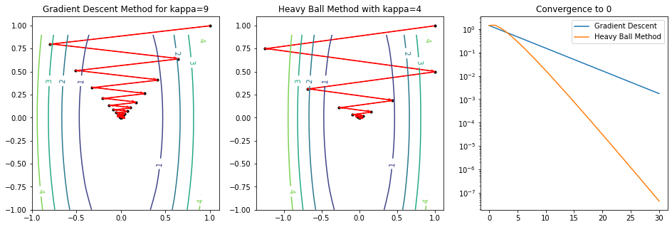
Consider the case where $A = \text{diag}(9,1)$, i.e., $f(x_1, x_2) = (9x_1^2+x_2^2)/2, \kappa = 9$. Setting $x_0 = [1,1]^\top$ and $\eta = 1$, the trajectory of GD iterates is zigzagging. In addition, we apply the heavy ball method to solving this problem. It shows that the introduced momentum speeds up the convergence.
f = quadratic_function(d=2, A=np.array(([9,0],[0,1])))
alg1 = GD(f, x0=np.array([1.,1.]))
alg2 = HeavyBall(f, x0=np.array([1.,1.]))
eta1 = 1/5
eta2 = 1/4
gamma2 = 1/4

for t in range(30):
    alg1.update(eta1)
    alg2.update(eta2, gamma2)


err_GD = np.linalg.norm(alg1.trajectory, 2, 1)
err_HB = np.linalg.norm(alg2.trajectory, 2, 1)

x1 = np.arange(-1, 1, 0.1)
x2 = np.arange(-1, 1, 0.1)
X1, X2 = np.meshgrid(x1, x2)
Y = 4.5*X1**2 + 0.5*X2**2
fig, (ax1, ax2, ax3) = plt.subplots(1,3, figsize=(16, 5))
CS = ax1.contour(X1, X2, Y, levels=4)
ax1.clabel(CS, inline=True, fontsize=10)
ax1.set_title('Gradient Descent Method for kappa=9')

for t, x in enumerate(alg1.trajectory):
    ax1.scatter(x[0], x[1], s=10, c='black', marker='o')
    if t < len(alg1.trajectory)-1:
        x_next = alg1.trajectory[t+1]
        ax1.arrow(x[0], x[1], x_next[0]-x[0], x_next[1]-x[1], shape='right', color='r', width=0.01, length_includes_head=True)

CS = ax2.contour(X1, X2, Y, levels=4)
ax2.clabel(CS, inline=True, fontsize=10)
ax2.set_title('Heavy Ball Method with kappa=4')

for t, x in enumerate(alg2.trajectory):
    ax2.scatter(x[0], x[1], s=10, c='black', marker='o')
    if t < len(alg2.trajectory)-1:
        x_next = alg2.trajectory[t+1]
        ax2.arrow(x[0], x[1], x_next[0]-x[0], x_next[1]-x[1], shape='right', color='r', width=0.01, length_includes_head=True)

t = np.arange(31)
ax3.plot(t, err_GD, label='Gradient Descent')
ax3.plot(t, err_HB, label='Heavy Ball Method')
ax3.legend()
ax3.set_title('Convergence to 0')
ax3.set_yscale('log')
f = quadratic_function(d=2, A=np.array(([9,0],[0,1])))
alg = NestrovAcc(f, x0=np.array([1.,1.]))
eta = 1/9

for t in range(30):
    alg.update(eta)

err_NestrovAcc = np.linalg.norm(alg.trajectory, 2, 1)

x1 = np.arange(-1, 1, 0.1)
x2 = np.arange(-1, 1, 0.1)
X1, X2 = np.meshgrid(x1, x2)
Y = 4.5*X1**2 + 0.5*X2**2
fig, (ax1, ax2) = plt.subplots(1,2, figsize=(12,5))
CS = ax1.contour(X1, X2, Y, levels=4)
ax1.clabel(CS, inline=True, fontsize=10)
ax1.set_title("Nestrov's Accelerated GD with kappa=9")

for t, x in enumerate(alg.trajectory):
    ax1.scatter(x[0], x[1], s=10, c='black', marker='o')
    if t < len(alg.trajectory)-1:
        x_next = alg.trajectory[t+1]
        ax1.arrow(x[0], x[1], x_next[0]-x[0], x_next[1]-x[1], shape='right', color='r', width=0.01, length_includes_head=True)


t = np.arange(31)
ax2.plot(t, err_GD, label='Gradient Descent')
ax2.plot(t, err_NestrovAcc, label="Nestrov's Accelerated GD")
ax2.legend()
ax2.set_title('Convergence to 0')
ax2.set_yscale('log')
f = quadratic_function(d=2, A=np.array(([1,0],[0,1])))
alg = SGD(f, x0=np.array([1.,1.]))
eta = 1

for t in range(5):
    alg.update(eta, sigma=0.1)

print(alg.trajectory)

x1 = np.arange(-1, 1, 0.1)
x2 = np.arange(-1, 1, 0.1)
X1, X2 = np.meshgrid(x1, x2)
Y = 0.5*X1**2 + 0.5*X2**2
fig, ax = plt.subplots()
CS = ax.contour(X1, X2, Y, levels=4)
ax.clabel(CS, inline=True, fontsize=10)
ax.set_title('Noisy Gradient Descent Method for kappa=1')
ax.scatter(0,0,s=20, c='red', marker='*')
for t, x in enumerate(alg.trajectory):
    ax.scatter(x[0], x[1], s=10, c='black', marker='o')
    if t < len(alg.trajectory)-1:
        x_next = alg.trajectory[t+1]
        ax.arrow(x[0], x[1], x_next[0]-x[0], x_next[1]-x[1], shape='right', color='r', width=0.01, length_includes_head=True)
[array([1., 1.]), array([0.05638466, 0.05660117]), array([-0.0959119 , -0.07248226]), array([-0.00137746, -0.11649844]), array([0.00086801, 0.21639027]), array([ 0.12597407, -0.02129214])]