STA 142A Statistical Learning I - Discussion 3 - Python
Some Packages
- numpy: The fundamental package for scientific computing with Python
- scikit-learn: Machine Learning in Python
- matploblib: Visualization with Python
- seaborn: Statistical data visualization
- statsmodels: statistical models, hypothesis tests, and data exploration
Array vs. Numpy Array
a = [1,2,3]
a * 3
[1, 2, 3, 1, 2, 3, 1, 2, 3]
a + 3
---------------------------------------------------------------------------

TypeError                                 Traceback (most recent call last)

<ipython-input-4-d390b6b495e8> in <module>
----> 1 a + 3


TypeError: can only concatenate list (not "int") to list
import numpy as np
b = np.array([1,2,3])
b * 3
array([3, 6, 9])
b + 3
array([4, 5, 6])
c = np.array([4,5,6])
b * c
array([ 4, 10, 18])
# 1d array
b.shape
(3,)
# 2d array
d1 = b.reshape(-1,1)
d1
array([[1],
       [2],
       [3]])
d1.shape
(3, 1)
d2 = b.reshape(1,-1)
d2
array([[1, 2, 3]])
d2.shape
(1, 3)
# matrix multiplication
d1 @ d2
array([[1, 2, 3],
       [2, 4, 6],
       [3, 6, 9]])
d2 @ d1
array([[14]])
Random Sampling
https://numpy.org/doc/stable/reference/random/index.html
from numpy.random import default_rng
rng = default_rng()
vals = rng.standard_normal(10)
vals
array([-0.77521747, -0.84113655,  0.61197545, -0.13576524,  0.70373505,
        0.61064352, -0.01271956, -0.29483544, -2.47983637,  1.08520542])
Linear Regression
import matplotlib.pyplot as plt
import seaborn as sns
n = 100
b0, b1 = 5, 3
# Generate X and epsilon
e = rng.normal(0,1,n)
X = rng.uniform(0,1,n)
Y = b0+b1*X+e
X = X.reshape(-1,1)
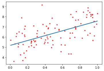
# Seaborn
sns.regplot(X, Y, ci=None, scatter_kws={'color':'r', 's':9})
plt.show()
# Sklearn
from sklearn import linear_model
from sklearn.metrics import mean_squared_error, r2_score
# Create linear regression object
regr = linear_model.LinearRegression()
# Train the model using the training sets
regr.fit(X, Y)
# Make predictions using the testing set
Y_pred = regr.predict(X)
# The coefficients
print('Coefficients: \n', regr.coef_)
# The mean squared error
print('Mean squared error: %.2f'
% mean_squared_error(Y, Y_pred))
# The coefficient of determination: 1 is perfect prediction
print('Coefficient of determination: %.2f'
% r2_score(Y, Y_pred))
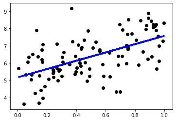
# Plot outputs
plt.scatter(X, Y, color='black')
plt.plot(X, Y_pred, color='blue', linewidth=3)
plt.show()
Coefficients:
 [2.40581767]
Mean squared error: 1.04
Coefficient of determination: 0.32