STA 142A Statistical Learning I

Discussion 8: A Short Tutorial in pyGAM

TA: Tesi Xiao

Recap

Generalized Additive Models (GAMs) are smooth semi-parametric models of the form:

where $X = [X_1, X_2, \dots, X_d]^\top, Y\in\mathbb{R}$, and $g()$ is the link function that relates the predictor variables to the conditioned expected value of $Y$.

The functions $f_i(\cdot)$ are built using penalized basis spline (B-spline), also known as P-spline, which can be interpreted as smoothing spline with specific basis functions. These functions $f_i$’s allow us to automatically model non-linear relationships without having to manually try out many different transformations on each variable.

In general, we can express all kinds of Generalized Additive Models in the form of

and

Remark. In general, each function $f_i$ in GAM can be a multi-variate function such as $f_i(X_p, X_q)$.

pyGAM

Create model instances

From the above formulation, we can see that a GAM consists of 3 components:

• distribution from the exponential family
• link function $g(\cdot)$
• function form with an additive structure $\beta_0 + f_1(X_1) + f_2(X_2) + \dots + f_d(X_d)$

In pyGAM, we can use

class pygam.pygam.GAM(terms='auto', max_iter=100, tol=0.0001, distribution='normal', link='identity', callbacks=['deviance', 'diffs'], fit_intercept=True, verbose=False, **kwargs)

to create a GAM specified by

• distribution: 'normal', 'binomial', 'poisson', 'gamma', 'inv_gauss'
• link: 'identity', 'logit', 'inverse', 'log', 'inverse-squared'
• terms: we can either choose ‘auto’ by default (without passing any argument to terms) os specify the functional form manually by passing an expression to terms. To be specific, we specify the functional form using terms: l() - linear terms; s() - spline terms; f() - factor terms; intercept.

Remark. Note that models include an intercept by default due to fit_intercept=True.

For example, if we want to fit a linear GAM (distribution='normal', link='identity') like

where $X_1, X_2$ are numeric variables, $X_3$ are binary-valued variables ($X_3=0,1$). Then we can build the model using GAM like:

from pygam import GAM, s, l, f

GAM(s(0) + l(1) + f(2))

GAM(callbacks=['deviance', 'diffs'], distribution='normal', 
   fit_intercept=True, link='identity', max_iter=100, 
   terms=s(0) + l(1) + f(2), tol=0.0001, verbose=False)

Remark.

1. distribution='normal', link='identity' and fit_intercept=True are already set by default. The index of the preditor variable starts at 0, i.e., $0 –> X_1; 1–>X_2; 2–>X_3$
2. we can also specify different arguments in terms s(), l(), and f(); see API. For instance, we can specify the order of basis functions and the penalty parameter lam in the B-spline term.

pygam.terms.s(feature, n_splines=20, spline_order=3, lam=0.6, penalties='auto', constraints=None, dtype='numerical', basis='ps', by=None, edge_knots=None, verbose=False)

In pyGAM, for convenience, you can build custom models by specifying these 3 elements, or you can choose from common models:

• LinearGAM identity link and normal distribution
• LogisticGAM logit link and binomial distribution
• PoissonGAM log link and Poisson distribution
• GammaGAM log link and gamma distribution
• InvGauss log link and inv_gauss distribution

Fit models

In pyGAM, you can either use .fit() or .gridsearch() to fit GAMs on the training set. The difference is that .gridsearch() performs a grid search over a space of all tunable parameters; see API. Thus, .gridsearch() is slow but may have better results.

from pygam import LinearGAM, s
from pygam.datasets import toy_interaction

X, y = toy_interaction(return_X_y=True)

gam = LinearGAM(s(0)).fit(X, y)
gam.summary()

LinearGAM                                                                                                 
=============================================== ==========================================================
Distribution:                        NormalDist Effective DoF:                                     19.1074
Link Function:                     IdentityLink Log Likelihood:                               -123123.6702
Number of Samples:                        50000 AIC:                                           246287.5553
                                                AICc:                                          246287.5722
                                                GCV:                                                4.1528
                                                Scale:                                                4.15
                                                Pseudo R-Squared:                                   0.0005
==========================================================================================================
Feature Function                  Lambda               Rank         EDoF         P > x        Sig. Code   
================================= ==================== ============ ============ ============ ============
s(0)                              [0.6]                20           19.1         9.06e-02     .           
intercept                                              1            0.0          8.54e-01                 
==========================================================================================================
Significance codes:  0 '***' 0.001 '**' 0.01 '*' 0.05 '.' 0.1 ' ' 1

WARNING: Fitting splines and a linear function to a feature introduces a model identifiability problem
         which can cause p-values to appear significant when they are not.

WARNING: p-values calculated in this manner behave correctly for un-penalized models or models with
         known smoothing parameters, but when smoothing parameters have been estimated, the p-values
         are typically lower than they should be, meaning that the tests reject the null too readily.

The method .predict(X) predicts expected value of target given model and input $X$. The method score(X, y, weights=None) is to compute the explained deviance for a trained model for a given $X$ and $y$.

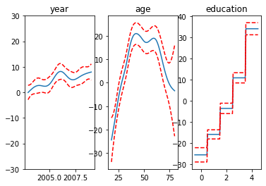
Visualize each function

from pygam import LinearGAM, s, f
from pygam.datasets import wage
import matplotlib.pyplot as plt

X, y = wage(return_X_y=True)

## model
gam = LinearGAM(s(0) + s(1) + f(2))
gam.gridsearch(X, y)


## plotting
plt.figure();
fig, axs = plt.subplots(1,3);

titles = ['year', 'age', 'education']
for i, ax in enumerate(axs):
    XX = gam.generate_X_grid(term=i)
    ax.plot(XX[:, i], gam.partial_dependence(term=i, X=XX))
    ax.plot(XX[:, i], gam.partial_dependence(term=i, X=XX, width=.95)[1], c='r', ls='--')
    if i == 0:
        ax.set_ylim(-30,30)
    ax.set_title(titles[i]);