STA 142A Statistical Learning I

Discussion 7: Introduction to Numerical Optimization

TA: Tesi Xiao

In general, an optimization problem can be formulated as

The function $f(x)$ is the objective function and the set $\mathcal{C}$ are called the constraint set. In particular, the stanford form of a continuous optimization problem is

where

• $f:\mathbb{R}^d \rightarrow \mathbb{R}$ is the objective function to be minimized over d-dimensional vector $x$
• $g_i(x)\leq 0$ are called inequality constraints
• $h_j(x)=0$ are called equality constraints
• $m, p \geq 0$
• Unconstrained vs. Constrained: If $m=p=0$ in the above formulation, then the problem is an unconstrained optimization problem. The constraint set $\mathcal{C} \equiv \mathbb{R}^d$.
• Convex vs. Non-convex:
  • When the objective function $f(x)$ is convex, the optimization problem above enjoys certain property: the minimum value either is obtained at the point $\nabla f(x)=0$ or on the boundary of the constraint set $\mathcal{C}$.
  • If the objective function $f(x)$ is non-convex (not convex), the optimization problem can be complicated with different local minima and the global minimum point can be so hard to find.

Question: Why we need to investigate optimization algorithms for solving problems above?

For most cases, a closed-form solution $x^\star = \underset{x\in\mathcal{C}}{\arg\min}~ f(x)$ is unable to find, even in the convex setting. For example, in Linear Regression, we know that $\hat{\beta} = \arg\min~ \Vert Y-X\beta \Vert^2 = (X^\top X)^{-1} X^\top Y$. The objective function $\Vert Y-X\beta \Vert^2$ here is a convex function of $\beta$. However, for Logistic Regression, $\hat{\beta} = \arg\min~\sum_{i=1}^{n} \log (1+\exp^{-y_i (x_i^\top \beta)})$ does not has an explicit expression, even though the logistic loss here is convex. Therefore, for these cases, we aim to find the approximate solution by some algorithms.

Uniform Grid Method

The naive algorithm is the uniform grid method. In the 1-d case, assume we know a rough interval $[L,R]$ that contains the optimal solution. Then, we can form a grid with $N$ points uniformly on this interval $[L,R]$. Check all the function values of these points and return the one with the smallest function value. However, this method has certain limitations:

• The uniform grid approach requires the prior information of $x^\star$. In the unconstrained setting, it may be hard to find such an interval containing the optimal solution.
• The curse of dimensionality: In the 1-d cases, the above method is simply to check $N$ different points on $[L,R]$. However, when the dimension $d$ increases, the number of points to check is growing in the order of $N^d$.
• The above method faild to leverage the property of $f(x)$.

First-order Method: Gradient Descent

Assume $f(x)$ is convex and $f’(x)$ is its derivative. The Gradient Descent (GD) algorithm moves the iterate along the negative gradient direction at each step.

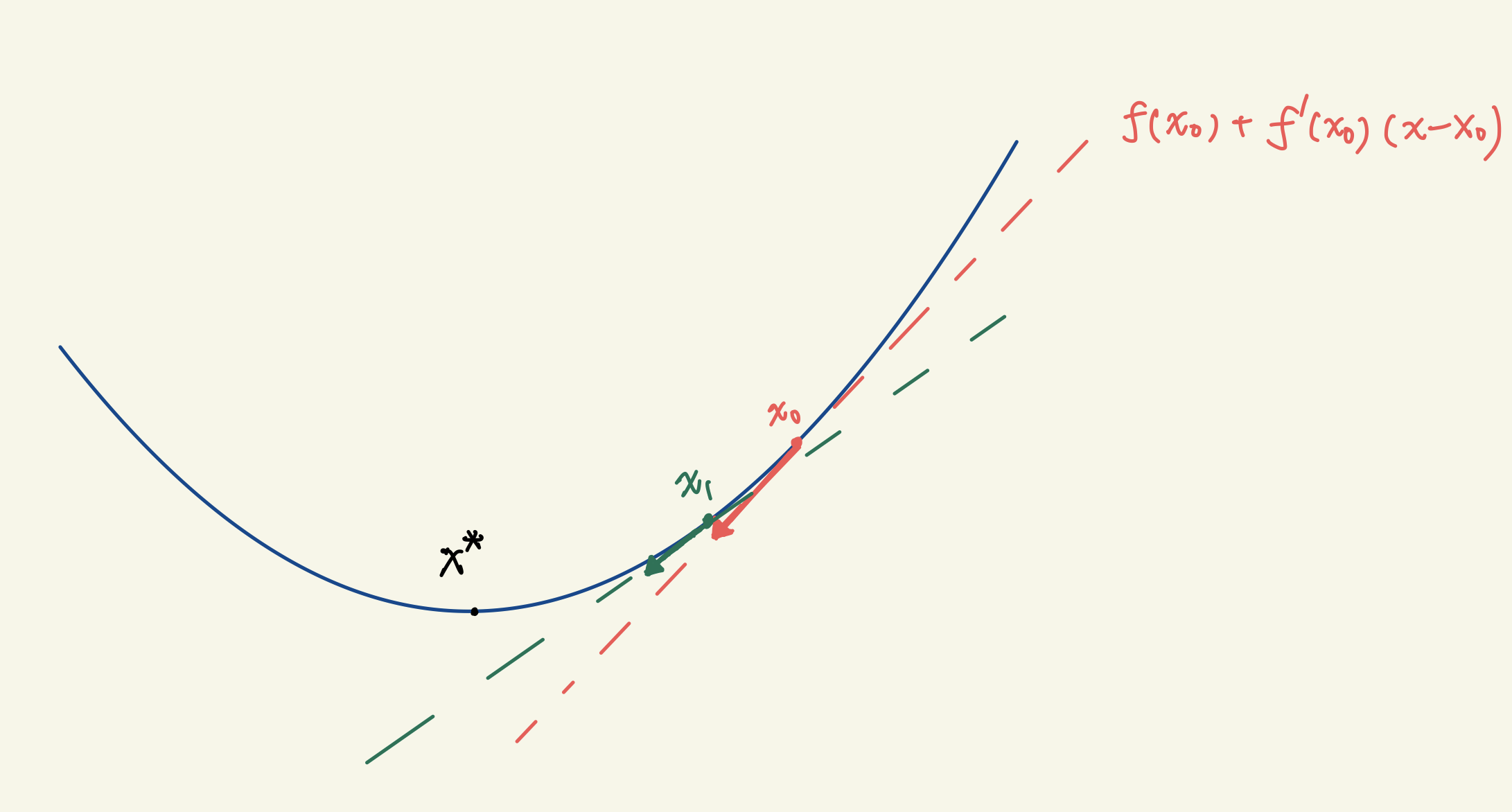
One can show that the iterate generated by GD converge to the optimal solution $x^\star$ when the objective function $f(x)$ is strongly-convex.

Remark

• GD is also commonly used for solving non-convex problems to find some local minima.
• $f’‘(x)$ (the curvature of $f(x)$) can also be utilized to find $x^\star$. These algorithms are calls Second-order Methods. For example, Newton’s method.