STA 142A Statistical Learning I
Discussion 5: Classification Methods: Logistic Regression, LDA, QDA, SVM
TA: Tesi Xiao
In this session, we will focus on 4 different binary classification methods: Linear Regression, Linear/Qudratic Discriminative Analysis, and Support Vector Machine.
Recall that the Bayes optimal classifier is given by
\[f^\star (x) = \begin{cases} 1, & \text{if } \eta(x)\geq 1/2\\ -1, & \text{if } \eta(x) < 1/2\end{cases} = \text{sign}\bigg(\log \frac{\eta(x)}{1-\eta(x)}\bigg),\]where $\eta(x)= P(Y=1 \vert X=x)$.
However, in general, $\eta(x)$ is unknown since no one knows the underlying joint distribution of $(X, Y)$ given the observed sample. In order to construct a classifier, we need to find ways of modeling the joint distribution $P(X, Y)$.
Note that
\[P(X, Y) = P(Y|X) P(X) = P(X|Y) P(Y).\]Thus, there are 2 approaches to formulate the model:
- (Discriminative Approach) Model $P(Y\vert X)$ directly: In this case, we don’t care about how $X$ is distributed. We assume that $\hat{P}(Y\vert X)$ can approximate the true $P(Y\vert X)$. Then, the function $\hat{\eta}(x)$, an approximation of $\eta(x)$ can be obtained immediately to find a classfier $\hat{f}$ in the form of $f^\star$. For example, Logistic Regression and SVM.
- (Generative Approach) Model $P(Y)$ and $P(X\vert Y)$: In this case, we actually pay attention to what is the proportion of postive samples and negative samples, i.e., $P(Y)$, and how $X$ is distributed within each class, i.e., $P(X\vert Y)$. For example, LDA and QDA.
Logistic Regression
In Logistic Regression, we aim to directly provide a parametrized function for $P(Y\vert X)$. To be specific, we approximate $P(Y\vert X)$ by
\[P_{\beta}(Y=1|X=x) = \frac{1}{1+\exp (-x^\top \beta)} = \eta_{\beta}(x).\]- Odds Ratio = $\frac{P(Y=1\vert X=x)}{P(Y=-1\vert X=x)} = \frac{\eta(x)}{1-\eta(x)} = \exp (x^\top\beta)$
- Log-odds Ratio = $x^\top \beta$
In this case, the Bayes Optimal Classifier for $\eta_{\beta}(x)$ is given by
\[f^\star_{\beta}(x) = \begin{cases}1, &\text{if } x^\top\beta\geq0\\-1, &\text{if } x^\top\beta<0\end{cases} = \text{sign}(x^\top\beta)\]It is natural to ask how to find the value of $\beta$ in practice given the training data ${(x_i, y_i)}_{i=1,\dots,n}$. The answer is MLE. The MLE of $\beta$ is given by
\[\begin{aligned}\hat{\beta}_n &= \underset{\beta}{\arg\max}~\ell(\beta) = \underset{\beta}{\arg\max}~ \sum_{i=1}^{n} \log P_{\beta} (Y=y_i |X=x_i) + \sum_{i=1}^{n} \log P(X=x_i)\\ &= \underset{\beta}{\arg\max}~ \sum_{i=1}^{n} \log P_{\beta} (Y=y_i |X=x_i)\\ &= \underset{\beta}{\arg\max}~ -\sum_{i=1}^{n} \log (1+\exp (-y_i \cdot x_i^\top \beta))\\ &= \underset{\beta}{\arg\min}~ \sum_{i=1}^{n} \log (1+\exp (-y_i \cdot x_i^\top \beta)) \rightarrow \text{Logistic Loss}. \end{aligned}\]Linear/Qudratic Discriminative Analysis
In LDA/QDA, we attempt to model how the data is generated. We assume that the data come from a Gaussian Mixture Model. In binary classification problem, it means that $X\vert Y=1$ and $X\vert Y=-1$ follow two Gaussian distribution respectively. We will illustrate it with 1-d cases below.
1. QDA
Assume that $P(Y=1) = \pi_1, P(Y=-1) = \pi_{-1} = 1-\pi_1$ and $X\vert Y=1\sim N(\mu_1, \sigma_1^2), X\vert Y=-1\sim N(\mu_{-1}, \sigma_{-1}^2)$ ($\sigma_1 \neq \sigma_{-1}$). Note that
\[\eta(x) = P(Y=1|X=x) = \frac{P(Y=1, X=x)}{P(X=x)} = \frac{P(X=x|Y=1)P(Y=1)}{P(X=x)}\] \[1-\eta(x) = \frac{P(X=x|Y=-1)P(Y=-1)}{P(X=x)}\]Thus,
\[\begin{aligned}\frac{\eta(x)}{1-\eta(x)} &= \frac{P(X=x|Y=1)\pi_1}{ P(X=x|Y=-1)\pi_{-1}}\\ &= \frac{\pi_1 \sigma_1^{-1} \exp (-\frac{(x-\mu_1)^2}{2\sigma_1^2})}{\pi_{-1} \sigma_{-1}^{-1} \exp (-\frac{(x-\mu_{-1})^2}{2\sigma_{-1}^2})}\\ &= \frac{\pi_1\sigma_1^{-1}}{\pi_{-1}\sigma_{-1}^{-1}}\cdot \exp \left\{ -\frac{(x-\mu_1)^2}{2\sigma_1^2} + \frac{(x-\mu_{-1})^2}{2\sigma_{-1}^2}\right\}\end{aligned}\]and
\[\log \frac{\eta(x)}{1-\eta(x)} = -\frac{(x-\mu_1)^2}{2\sigma_1^2} + \frac{(x-\mu_{-1})^2}{2\sigma_{-1}^2} + \log \frac{\pi_1\sigma_1^{-1}}{\pi_{-1}\sigma_{-1}^{-1}} = \text{RHS}\]is a qudratic function of $x$. In this case, the Bayes optimal classifier for this Gaussian mixture model is
\[f^\star (x) = \begin{cases} 1, & \text{if RHS}\geq0 \\ -1, & \text{if RHS} < 0\end{cases} = \text{sign}\bigg(\log \frac{\eta(x)}{1-\eta(x)}\bigg).\]2. LDA
LDA is a special case of QDA with $\sigma_1 = \sigma_{-1} = \sigma$, In this case,
\[\text{RHS} = \frac{-(x-\mu_1)^2+ (x-\mu_{-1})^2}{2\sigma^2} + \log \frac{\pi_1}{\pi_{-1}}= \frac{\mu_1 -\mu_{-1}}{\sigma^2}\cdot (x-\frac{\mu_1 + \mu_{-1}}{2}) + \log \frac{\pi_1}{\pi_{-1}}\]is a linear function of $x$. The decision boundary is the value of $x$ when $\text{RHS}=0$. For example, in LDA when $\pi_1=\pi_{-1}$, the decision boundary is $x=\frac{\mu_1 + \mu_{-1}}{2}$. In general, QDA provides a quadratic decision boundary and LDA gives a linear decision boundary.
Remark. Note that in LDA and QDA, $\beta=(\pi_1, \pi_{-1}, \mu_1, \mu_{-1}, \sigma_1, \sigma_{-1})$ are the unknown model parameters. Similar to Logistic Regression, we obtain its estimate by MLE. Assume we observe that
\[Y=1: x_1^{(1)}, x_1^{(2)}, \dots, x_{1}^{(n_1)} \text{ and }Y=-1: x_{-1}^{(1)}, x_{-1}^{(2)}, \dots, x_{-1}^{(n_{-1})}\]Then
\[\hat{\pi}_1 = \frac{n_1}{n_1 + n_{-1}}, \quad \hat{\pi}_{-1} = \frac{n_{-1}}{n_1 + n_{-1}}\] \[\hat{\mu}_1 = \bar{x}_1 = \frac{1}{n_1} \sum_{i=1}^{n_1} x_{1}^{(i)}, \quad \hat{\mu}_{-1} = \bar{x}_{-1} = \frac{1}{n_{-1}} \sum_{i=1}^{n_{-1}} x_{-1}^{(i)}\] \[\hat{\sigma}_1^2 = \frac{1}{n_1} \sum_{i=1}^{n_1} (x_1^{(i)} - \bar{x}_1)^2, \quad \hat{\sigma}_{-1}^2 = \frac{1}{n_{-1}} \sum_{i=1}^{n_{-1}} (x_{-1}^{(i)} - \bar{x}_{-1})^2\]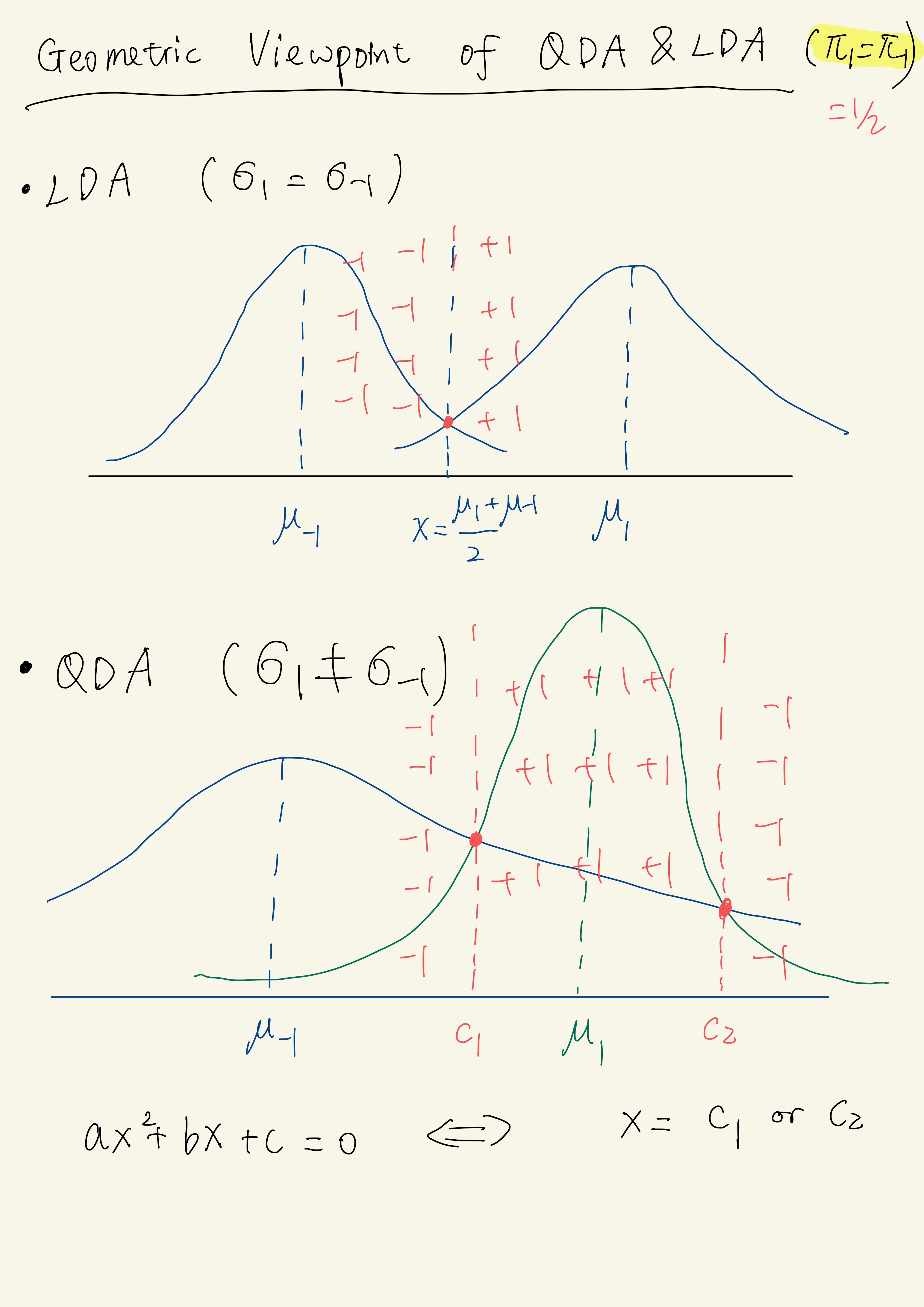
Support Vector Machine
See the hand-written notes here