STA 141C Big-data and Statistical Computing
Discussion 7: Support Vector Machine
TA: Tesi Xiao
Linear SVM
Linear SVM treats training examples as points in the Euclidean space and finds support vectors that maximise the width of the gap between the two classes.
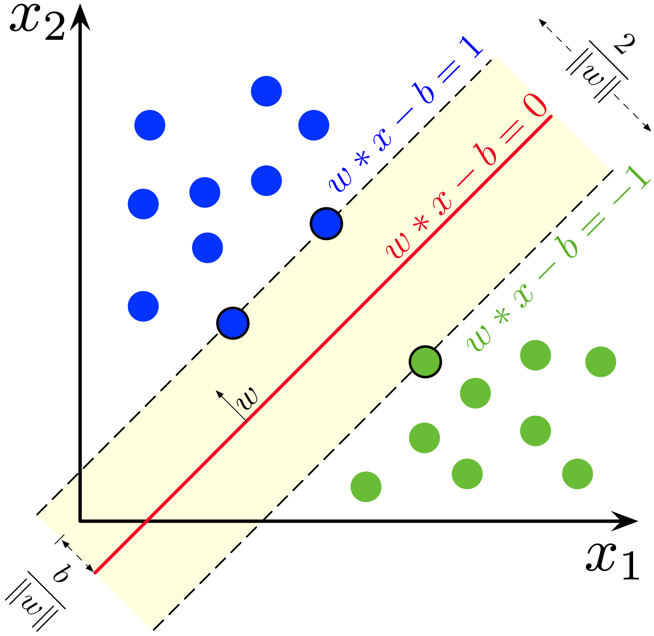
(Image Source: Wikipedia)
- Pros:
- Effective in high dimensional spaces
- Uses a subset of training points in the decision function (called support vectors), so it is also memory efficient.
- Cons:
- Linear SVM only provides linear decision boundary
- Overfitting issues when the number of features is much greater than the number of samples
To address the disadvantages of linear SVM, kernel tricks are crucial.
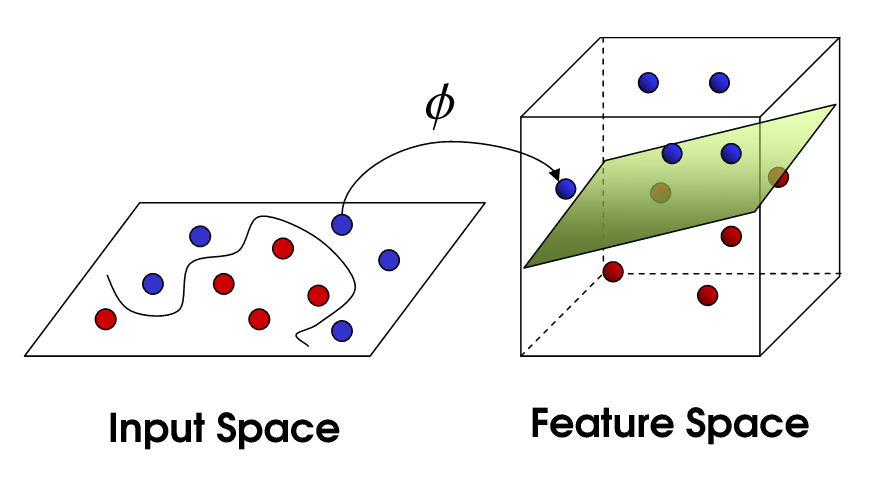
Kernel SVM
Kernel SVM maps training examples with function $\phi$ to points in a new space and then maximise the width of the gap between the two classes
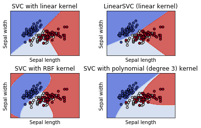
# Code from

import numpy as np
import matplotlib.pyplot as plt
from sklearn import svm, datasets


def make_meshgrid(x, y, h=.02):
    """Create a mesh of points to plot in

    Parameters
    ----------
    x: data to base x-axis meshgrid on
    y: data to base y-axis meshgrid on
    h: stepsize for meshgrid, optional

    Returns
    -------
    xx, yy : ndarray
    """
    x_min, x_max = x.min() - 1, x.max() + 1
    y_min, y_max = y.min() - 1, y.max() + 1
    xx, yy = np.meshgrid(np.arange(x_min, x_max, h),
                         np.arange(y_min, y_max, h))
    return xx, yy


def plot_contours(ax, clf, xx, yy, **params):
    """Plot the decision boundaries for a classifier.

    Parameters
    ----------
    ax: matplotlib axes object
    clf: a classifier
    xx: meshgrid ndarray
    yy: meshgrid ndarray
    params: dictionary of params to pass to contourf, optional
    """
    Z = clf.predict(np.c_[xx.ravel(), yy.ravel()])
    Z = Z.reshape(xx.shape)
    out = ax.contourf(xx, yy, Z, **params)
    return out


# import some data to play with
iris = datasets.load_iris()
# Take the first two features. We could avoid this by using a two-dim dataset
X = iris.data[:, :2]
y = iris.target

# we create an instance of SVM and fit out data. We do not scale our
# data since we want to plot the support vectors
C = 1.0  # SVM regularization parameter
models = (svm.SVC(kernel='linear', C=C),
          svm.LinearSVC(C=C, max_iter=10000),
          svm.SVC(kernel='rbf', gamma=0.7, C=C),
          svm.SVC(kernel='poly', degree=3, gamma='auto', C=C))
models = (clf.fit(X, y) for clf in models)

# title for the plots
titles = ('SVC with linear kernel',
          'LinearSVC (linear kernel)',
          'SVC with RBF kernel',
          'SVC with polynomial (degree 3) kernel')

# Set-up 2x2 grid for plotting.
fig, sub = plt.subplots(2, 2)
plt.subplots_adjust(wspace=0.4, hspace=0.4)

X0, X1 = X[:, 0], X[:, 1]
xx, yy = make_meshgrid(X0, X1)

for clf, title, ax in zip(models, titles, sub.flatten()):
    plot_contours(ax, clf, xx, yy,
                  cmap=plt.cm.coolwarm, alpha=0.8)
    ax.scatter(X0, X1, c=y, cmap=plt.cm.coolwarm, s=20, edgecolors='k')
    ax.set_xlim(xx.min(), xx.max())
    ax.set_ylim(yy.min(), yy.max())
    ax.set_xlabel('Sepal length')
    ax.set_ylabel('Sepal width')
    ax.set_xticks(())
    ax.set_yticks(())
    ax.set_title(title)

plt.show()
Comparing SVMs with logistic regression
- Logistic regression outputs probability estimates.
- SVMs do not directly provide probability estimates, these are calculated using an expensive five-fold cross-validation (see Scores and probabilities).