STA 141C Big-data and Statistical Computing

Discussion 3: Kernel PCA

TA: Tesi Xiao

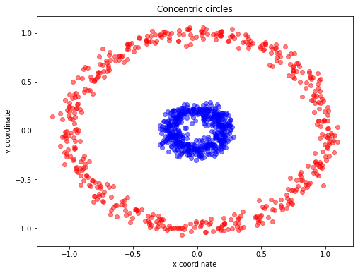
PCA is used to decompose a multivariate dataset in a set of successive orthogonal components that explain a maximum amount of the variance by using matrix factorization. Let start with a simple example of concentric circles.

from sklearn.datasets import make_circles
import matplotlib.pyplot as plt

X, y = make_circles(n_samples=1000, random_state=123, noise=0.05, factor=0.2) ## https://scikit-learn.org/stable/modules/generated/sklearn.datasets.make_circles.html

plt.figure(figsize=(8,6))

plt.scatter(X[y==0, 0], X[y==0, 1], color='red', alpha=0.5)
plt.scatter(X[y==1, 0], X[y==1, 1], color='blue', alpha=0.5)
plt.title('Concentric circles')
plt.ylabel('y coordinate')
plt.xlabel('x coordinate')
plt.show()

png

X, y

(array([[-0.08151124,  1.04156863],
        [-0.83407705,  0.55209298],
        [ 0.80292992,  0.49964037],
        ...,
        [ 0.18491366, -0.99335733],
        [-0.13239409, -0.99601977],
        [ 0.06469843,  0.05997449]]),
 array([0, 0, 0, 1, 0, 1, 0, 0, 1, 0, 0, 0, 0, 0, 0, 0, 1, 0, 0, 0, 0, 0,
        0, 1, 1, 1, 1, 0, 1, 0, 1, 0, 1, 0, 1, 1, 0, 0, 0, 1, 1, 0, 1, 0,
        1, 1, 0, 1, 0, 0, 0, 1, 1, 1, 0, 0, 1, 0, 1, 0, 1, 1, 0, 1, 0, 1,
        1, 1, 1, 0, 0, 1, 1, 0, 1, 1, 1, 1, 0, 1, 0, 0, 1, 0, 1, 0, 1, 1,
        0, 0, 1, 1, 1, 0, 0, 1, 1, 1, 1, 1, 1, 1, 1, 1, 1, 1, 0, 1, 1, 0,
        1, 1, 0, 0, 0, 0, 1, 1, 0, 1, 1, 1, 0, 1, 1, 0, 1, 0, 0, 0, 1, 0,
        1, 0, 0, 1, 1, 0, 1, 1, 0, 1, 0, 0, 0, 1, 1, 0, 1, 0, 1, 0, 1, 1,
        0, 1, 0, 0, 0, 1, 0, 1, 0, 0, 0, 0, 1, 0, 0, 0, 1, 1, 1, 1, 1, 0,
        1, 0, 1, 0, 0, 0, 1, 0, 0, 1, 1, 0, 0, 1, 0, 0, 1, 1, 0, 0, 0, 1,
        0, 0, 1, 1, 1, 1, 0, 1, 0, 0, 1, 0, 0, 1, 1, 0, 1, 1, 1, 0, 1, 0,
        1, 1, 0, 1, 0, 1, 0, 1, 1, 0, 0, 1, 0, 1, 0, 0, 0, 1, 0, 0, 1, 1,
        1, 0, 0, 1, 0, 0, 1, 0, 1, 1, 0, 0, 0, 0, 1, 0, 1, 0, 0, 1, 1, 0,
        0, 0, 0, 1, 0, 0, 0, 1, 1, 1, 0, 0, 1, 0, 1, 1, 1, 0, 1, 0, 0, 1,
        0, 1, 1, 1, 1, 1, 1, 1, 0, 1, 1, 0, 1, 0, 0, 0, 0, 0, 0, 1, 0, 0,
        0, 1, 1, 0, 0, 0, 0, 0, 0, 0, 0, 1, 0, 1, 0, 0, 1, 0, 1, 0, 0, 1,
        1, 1, 1, 0, 1, 1, 1, 1, 0, 1, 1, 0, 1, 0, 1, 1, 0, 0, 1, 0, 0, 1,
        1, 0, 0, 0, 1, 0, 0, 1, 0, 0, 0, 1, 1, 0, 1, 0, 1, 0, 0, 0, 0, 1,
        0, 1, 0, 1, 1, 0, 1, 1, 1, 1, 0, 0, 0, 0, 0, 0, 1, 0, 1, 1, 1, 1,
        0, 0, 0, 0, 0, 0, 1, 0, 1, 1, 1, 1, 1, 0, 0, 1, 0, 0, 0, 0, 1, 1,
        0, 0, 1, 0, 1, 1, 0, 0, 0, 1, 1, 1, 1, 1, 0, 0, 1, 0, 1, 1, 0, 0,
        1, 1, 0, 1, 0, 1, 0, 1, 0, 1, 1, 0, 0, 0, 1, 1, 1, 1, 1, 1, 1, 1,
        0, 0, 0, 0, 1, 1, 1, 0, 1, 1, 1, 0, 0, 1, 0, 1, 1, 0, 0, 1, 1, 1,
        0, 1, 0, 1, 0, 0, 1, 1, 1, 0, 0, 1, 0, 0, 1, 0, 1, 1, 0, 0, 0, 0,
        1, 0, 0, 1, 1, 1, 0, 1, 1, 0, 1, 0, 1, 1, 0, 0, 1, 0, 0, 1, 1, 1,
        0, 1, 0, 1, 1, 0, 1, 1, 0, 0, 0, 0, 1, 0, 1, 1, 1, 1, 0, 0, 0, 0,
        0, 1, 1, 0, 0, 1, 1, 1, 1, 1, 0, 1, 1, 0, 1, 1, 1, 0, 1, 1, 0, 1,
        0, 0, 1, 0, 1, 0, 0, 0, 1, 1, 1, 0, 1, 1, 0, 0, 0, 0, 0, 1, 0, 0,
        1, 1, 1, 1, 1, 0, 0, 0, 0, 1, 1, 0, 1, 1, 1, 1, 1, 1, 1, 0, 1, 0,
        0, 1, 1, 1, 0, 1, 0, 1, 0, 1, 1, 1, 1, 0, 1, 0, 0, 0, 1, 1, 1, 0,
        1, 1, 1, 1, 1, 0, 1, 1, 0, 1, 1, 0, 0, 0, 1, 1, 0, 1, 1, 0, 1, 1,
        0, 1, 0, 0, 0, 0, 1, 0, 0, 0, 1, 1, 1, 0, 0, 0, 0, 0, 1, 0, 0, 0,
        1, 1, 1, 1, 0, 1, 1, 0, 1, 0, 1, 0, 1, 0, 1, 0, 0, 0, 0, 0, 1, 1,
        1, 1, 0, 1, 0, 0, 0, 1, 1, 0, 1, 0, 1, 1, 0, 1, 0, 0, 0, 0, 1, 0,
        0, 1, 1, 1, 1, 0, 1, 0, 1, 1, 1, 1, 1, 1, 1, 0, 1, 1, 1, 1, 0, 1,
        1, 0, 0, 0, 1, 0, 1, 0, 1, 1, 1, 0, 0, 1, 0, 0, 1, 0, 1, 1, 1, 1,
        1, 0, 0, 0, 0, 0, 1, 1, 0, 0, 0, 1, 1, 1, 1, 1, 1, 0, 1, 1, 1, 0,
        1, 1, 1, 0, 0, 1, 1, 1, 1, 0, 1, 0, 0, 1, 1, 1, 0, 1, 0, 1, 1, 0,
        1, 0, 1, 0, 0, 1, 1, 1, 0, 1, 0, 0, 0, 1, 0, 1, 0, 0, 0, 0, 0, 1,
        1, 0, 0, 0, 0, 0, 1, 1, 1, 0, 1, 0, 0, 0, 1, 0, 0, 1, 0, 0, 1, 0,
        0, 1, 0, 0, 0, 0, 1, 0, 0, 1, 0, 1, 1, 1, 1, 0, 1, 1, 0, 0, 0, 0,
        0, 0, 0, 0, 0, 1, 0, 0, 0, 0, 1, 0, 1, 0, 0, 1, 0, 0, 0, 1, 1, 0,
        1, 0, 1, 1, 0, 1, 0, 1, 1, 0, 0, 1, 0, 0, 0, 0, 1, 0, 1, 0, 0, 1,
        1, 1, 0, 1, 1, 0, 0, 0, 1, 1, 0, 1, 0, 1, 1, 1, 1, 1, 1, 1, 0, 0,
        1, 1, 0, 1, 0, 0, 1, 0, 0, 1, 0, 0, 1, 1, 1, 1, 1, 0, 0, 0, 0, 1,
        1, 0, 0, 1, 0, 0, 1, 0, 0, 0, 0, 1, 1, 0, 0, 1, 0, 0, 1, 0, 1, 0,
        0, 1, 0, 1, 0, 1, 0, 0, 0, 1]))

For Kernel PCA, we can choose the kernel which is the best to decribe the underlying structure. One can interpret the kernel function as a measure of pairwise distance/similariry.

Below are several commonly used kernels. Also see user guide.

Cosine similarity

cosine_similarity computes the L2-normalized dot product of vectors. That is, if $x$ and $y$ are row vectors, their cosine similarity $k$ is defined as:

\[k(x, y) = \frac{x y^\top}{\|x\| \|y\|}\]

This is called cosine similarity, because Euclidean (L2) normalization projects the vectors onto the unit sphere, and their dot product is then the cosine of the angle between the points denoted by the vectors.

Linear kernel

The function linear_kernel computes the linear kernel, that is, a special case of polynomial_kernel with degree=1 and coef0=0 (homogeneous). If $x$ and $y$ are column vectors, their linear kernel is:

\[k(x, y) = x^\top y\]

Remark: Linear Kernel PCA = Standard PCA

Polynomial kernel

The function polynomial_kernel computes the degree-d polynomial kernel between two vectors. The polynomial kernel represents the similarity between two vectors. Conceptually, the polynomial kernels considers not only the similarity between vectors under the same dimension, but also across dimensions. When used in machine learning algorithms, this allows to account for feature interaction.

The polynomial kernel is defined as:

\[k(x, y) = (\gamma x^\top y +c_0)^d\]

where:

$x$, $y$ are the input vectors
$d$ is the kernel degree

If $c_0 = 0$ the kernel is said to be homogeneous.

Sigmoid kernel

The function sigmoid_kernel computes the sigmoid kernel between two vectors. The sigmoid kernel is also known as hyperbolic tangent, or Multilayer Perceptron (because, in the neural network field, it is often used as neuron activation function). It is defined as:

\[k(x, y) = \tanh( \gamma x^\top y + c_0)\]

where:

$x$, $y$ are the input vectors
$\gamma$ is known as slope
$c_0$ is known as intercept

RBF kernel

The function rbf_kernel computes the radial basis function (RBF) kernel between two vectors. This kernel is defined as:

\[k(x, y) = \exp( -\gamma \| x-y \|^2)\]

where $x$ and $y$ are the input vectors. If $\gamma = \sigma^{-2}$ the kernel is known as the Gaussian kernel of variance $\sigma^2$.

Laplacian kernel

The function laplacian_kernel is a variant on the radial basis function kernel defined as:

\[k(x, y) = \exp( -\gamma \| x-y \|_1)\]

where $x$ and $y$ are the input vectors and $|x-y|_1$ is the Manhattan distance between the input vectors.

from sklearn.decomposition import PCA, KernelPCA

## PCA fitting
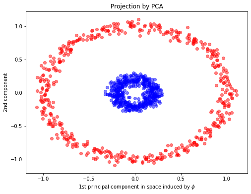
pca = PCA(n_components=2)
X_pca = pca.fit_transform(X)

## Kernel PCA fitting
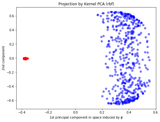
kpca = KernelPCA(n_components=2,kernel="rbf", fit_inverse_transform=True, gamma=10)
X_kpca = kpca.fit_transform(X)


plt.figure(figsize=(8,6))
plt.scatter(X_pca[y==0, 0], X_pca[y==0, 1], color='red', alpha=0.5)
plt.scatter(X_pca[y==1, 0], X_pca[y==1, 1], color='blue', alpha=0.5)
plt.xlabel(r"1st principal component in space induced by $\phi$")
plt.ylabel("2nd component")
plt.title("Projection by PCA")

Text(0.5, 1.0, 'Projection by PCA')

png

plt.figure(figsize=(8,6))
plt.scatter(X_kpca[y==0, 0], X_kpca[y==0, 1], color='red', alpha=0.5)
plt.scatter(X_kpca[y==1, 0], X_kpca[y==1, 1], color='blue', alpha=0.5)
plt.xlabel(r"1st principal component in space induced by $\phi$")
plt.ylabel("2nd component")
plt.title("Projection by Kernel PCA (rbf)")

Text(0.5, 1.0, 'Projection by Kernel PCA (rbf)')

png

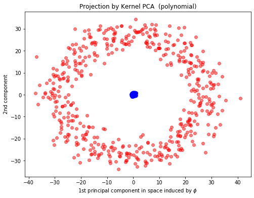
kpca_poly = KernelPCA(n_components=2,kernel="poly", fit_inverse_transform=True, gamma=10)
X_kpca_poly = kpca_poly.fit_transform(X)

plt.figure(figsize=(8,6))
plt.scatter(X_kpca_poly[y==0, 0], X_kpca_poly[y==0, 1]+0.02, color='red', alpha=0.5)
plt.scatter(X_kpca_poly[y==1, 0], X_kpca_poly[y==1, 1]-0.02, color='blue', alpha=0.5)
plt.xlabel(r"1st principal component in space induced by $\phi$")
plt.ylabel("2nd component")
plt.title("Projection by Kernel PCA  (polynomial)")

Text(0.5, 1.0, 'Projection by Kernel PCA  (polynomial)')

png

kpca_cos = KernelPCA(n_components=2,kernel="cosine", fit_inverse_transform=True, gamma=10)
X_kpca_cos = kpca_cos.fit_transform(X)

plt.figure(figsize=(8,6))
plt.scatter(X_kpca_cos[y==0, 0], X_kpca_cos[y==0, 1]+0.02, color='red', alpha=0.5)
plt.scatter(X_kpca_cos[y==1, 0], X_kpca_cos[y==1, 1]-0.02, color='blue', alpha=0.5)
plt.xlabel(r"1st principal component in space induced by $\phi$")
plt.ylabel("2nd component")
plt.title("Projection by Kernel PCA  (cosine)")

Text(0.5, 1.0, 'Projection by Kernel PCA  (cosine)')

png

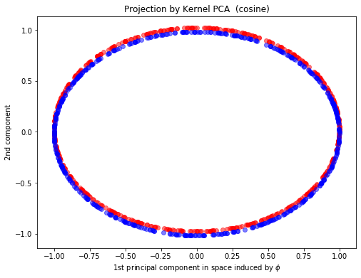
Feel free to try different kernels to see the impact brought by kernels.

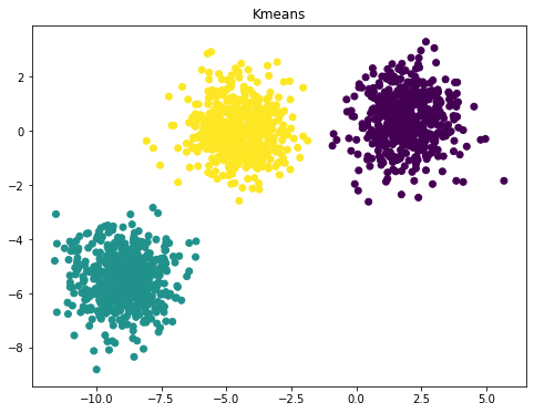
An example of K means clustering and RBF Kernel PCA

from sklearn.cluster import KMeans
from sklearn.datasets import make_blobs

n_samples = 1500
random_state = 170
X, y = make_blobs(n_samples=n_samples, random_state=random_state)

y_pred = KMeans(n_clusters=3, random_state=random_state).fit_predict(X)
plt.figure(figsize=(8,6))
plt.scatter(X[:, 0], X[:, 1], c=y_pred)
plt.title("Kmeans")

Text(0.5, 1.0, 'Kmeans')

png

kpca = KernelPCA(n_components=2,kernel="rbf", fit_inverse_transform=True, gamma=10)
X_kpca = kpca.fit_transform(X)
plt.figure(figsize=(8,6))
plt.scatter(X_kpca[y==0, 0], X_kpca[y==0, 1], color='red', alpha=0.5)
plt.scatter(X_kpca[y==1, 0], X_kpca[y==1, 1], color='blue', alpha=0.5)
plt.scatter(X_kpca[y==2, 0], X_kpca[y==2, 1], color='yellow', alpha=0.5)
plt.xlabel(r"1st principal component in space induced by $\phi$")
plt.ylabel("2nd component")
plt.title("Projection by Kernel PCA")

Text(0.5, 1.0, 'Projection by Kernel PCA')

png

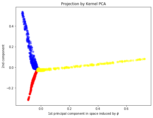
RBF kernel describes the affinity within the neighborhood. Thus, RBF Kernal PCA can recover the underlying blob-like clusters by the first two principle components.

word2vec

A detailed version of using word2vec on real data: https://github.com/kavgan/nlp-in-practice/blob/master/word2vec/Word2Vec.ipynb