STA 141C Big-data and Statistical Computing

Discussion 6: (Stochastic) Gradient Descent in Linear and Logistic Regression

TA: Tesi Xiao

Supervised vs Unsupervised Learning

The common tasks in unsupervised learning are clustering, representation learning (e.g. dimensionality reduction), and density estimation, in which we wish to learn the inherent structure of the data without using provided labels.
In supervised learning, we aim to explore the relations betweem predictors and responses (labels) usually for prediction purposes.

There are others regimes like semi-supervised learning, reinforcement learnng.

Emprical Risk Minimization (ERM)

Loss $L(y_{true}, y_{pred})$: a function to measure the loss value of predict the response/label of one observation $(x,y=y_{true})$ as $y_{pred} = f_\theta(x)$
Risk $R(f) = \mathbb{E}_{(x,y)} [L(y, f(x))]$: the expectation of loss function over the distribution of $(x,y)$.

In supervised learning, one can always formulate the goal is to find a function $f$ to minimize the risk $R(f)$. However, in most cases, we only observe a finite sample of datapoints from the population, i.e., $(x_1, y_1), \dots, (x_n, y_n)$. Therefore, we minimize the emprical risk (the avearge loss value) to find the function $f$.

\[\theta = \arg\min_{\theta} \frac{1}{n} \sum_{i=1}^n L(y_i, f_{\theta}(x_i))\]

Linear Regression: $f(x) = x^\top\theta,\quad \theta = \arg\min \frac{1}{n}\sum_{i=1}^n (y_i - x_i^\top \theta)^2$
Logistic Regression: $f(x) = e^{x^\top\theta}/(1+e^{x^\top\theta}),\quad \theta = \arg\min = \frac{1}{n} \sum_{i=1}^n \log (1+e^{-y_i x_i^\top \theta})$

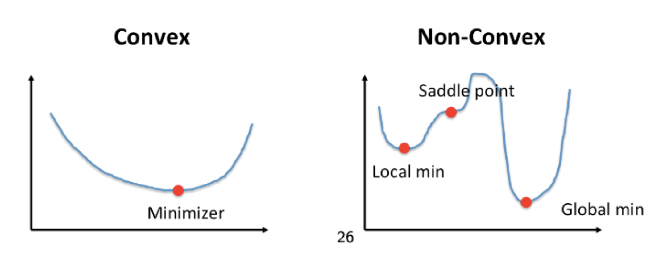
The ERM problems in linear and logistic regression are convex optimization problems.

Convex vs Non-convex Optimization

Linear Regression

Let’s implement the gradient descent algorithm to minimize the quadratic function $f(x) = \frac{1}{2} x^\top Q x + bx$. Note that the objective function in linear regression is a quaratic function of $\theta$.

import numpy as np
from numpy import random
import matplotlib.pyplot as plt
import pandas as pd

### function designed for gd on quadratic functions 0.5xQx - bx
## Q: positive definite matrix, n by n
## b: vector 1 by n
## x0: initial value
## T: stopping tolerance
## stepsize: stepsize for gd
## eps: converge tolerance
## trace: whether recording each updating
def gdQ(Q,b,x0 = None,T = 100,stepsize = 0.05,eps = 0.00001,trace = True):
    n = len(b)
    ## initialize
    if x0 is None:
        x0 = np.ones(n)
    ## recording iteration time
    start = 0
    x1 = x0 - stepsize*(np.dot(Q,x0)-b )
    ## recording each iteration
    if trace:
        x_trace = [x0,x1]
        eps_trace = [np.linalg.norm(x0-x1)]
    ## two stopping condition
    while( np.linalg.norm(x0-x1)>eps and start < T ):
        tmp = x1
        x1 = x1 - stepsize*(np.dot(Q,x1)-b )
        x0 = tmp
        if trace:
            x_trace.append(x1)
            eps_trace.append(np.linalg.norm(x0-x1))
        start += 1
    if trace:
        return x_trace,eps_trace
    else:
        return x1

n = 5
A = random.rand(n,n)
Q = np.dot(A,A.transpose())
b = 0.5*np.ones(n)
x_star,e = gdQ(Q,b)

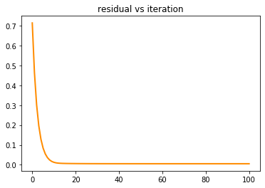
plt.figure()
lw = 2
x = np.arange(0,len(e),1)
plt.plot( x,e , color='darkorange',
         lw=lw)
plt.title('residual vs iteration')
plt.show()

png

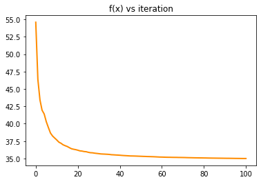
y_trace = [ 0.5*np.dot(np.dot(x.transpose(),Q),x)-np.dot(b,x)  for x in x_star]
plt.figure()
lw = 2
x = np.arange(0,len(y_trace),1)
plt.plot( x,y_trace , color='darkorange',
         lw=lw)
plt.title('f(x) vs iteration')
plt.show()

png

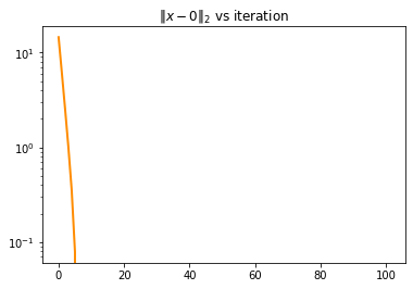
x_norm = [ np.linalg.norm(x)  for x in x_star]
plt.figure()
lw = 2
x = np.arange(0,len(x_norm),1)
plt.plot( x,y_trace , color='darkorange',
         lw=lw)
plt.yscale('log')
plt.title(r'$\Vert x - 0\Vert_2$ vs iteration')
plt.show()

png

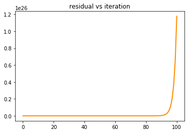
## a larger stepsize will not guarantee the converge
x_star,e = gdQ(Q,b,stepsize= 0.4)
plt.figure()
lw = 2
x = np.arange(0,len(e),1)
plt.plot( x,e , color='darkorange',
         lw=lw)
plt.title('residual vs iteration')
plt.show()

png

Logistic Regression

We then implement stochastic gradient descent for logistic regression.

import random
def F(X,y,w):
    n = np.size(y)
    F_value = 0
    for i in range(n):
        tmp = np.exp(-y[i]* np.dot(w,X[i]))
        F_value = F_value + np.log(1+tmp)
    return F_value

def GF_S(X,y,w,I):
    n = np.size(y)
    F_value = 0
    for i in I:
        tmp = np.exp(-y[i]* np.dot(w,X[i]))
        F_value = F_value -y[i]*X[i]*tmp/(1+tmp)
    return F_value
## sgd for above loss function
## mainly change the derivative function
def sgd_logistic(X,y,B = 10,x0 = None,T = 300,stepsize = 0.005,eps = 0.00001,trace = True):
    n = len(X[0])
    if x0 is None:
        x0 = 0.05*np.ones(n)
    start = 0
    I = random.sample(range(len(y)),B)
    x1 = x0 - stepsize*GF_S(X,y,x0,I)
    if trace:
        x_trace = [x0,x1]
        eps_trace = [np.linalg.norm(x0-x1)]
    while( np.linalg.norm(x0-x1)>eps and start < T ):
        I = random.sample(range(len(y)),B)
        tmp = x1
        x1 = x1 - stepsize*GF_S(X,y,x1,I)
        x0 = tmp
        if trace:
            x_trace.append(x1)
            eps_trace.append(np.linalg.norm(x0-x1))
        start += 1
    if trace:
        return x_trace,eps_trace
    else:
        return x1

from sklearn.datasets import load_iris
X, y = load_iris(return_X_y=True)
X, y = X[:100], y[:100]

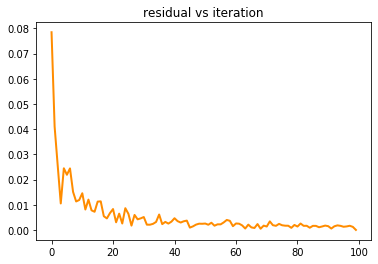
theta ,e = sgd_logistic(X,y)

plt.figure()
lw = 2
x = np.arange(0,len(e),1)
plt.plot( x,e , color='darkorange',
         lw=lw)
plt.title('residual vs iteration')
plt.show()

png

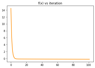
y_trace = [ F(X,y,w)  for w in theta]
plt.figure()
lw = 2
x = np.arange(0,len(y_trace),1)
plt.plot( x,y_trace , color='darkorange',
         lw=lw)
plt.title('f(x) vs iteration')
plt.show()

png